What if Justices Really Voted Their Values?

In my last two entries, I demonstrated that Segal/Cover scores are an especially directional set of preference assignments that declare some justices to have perfectly-extreme political views. For example, Antonin Scalia is said to have a reputation for perfect conservatism (-1). Through a roundabout way that I will not repeat here, however, I argued that when newspaper editorialists all agree that Scalia is conservative, they do so under the assumption that the political values in question will be expressed within the constraints of a pre-existing institutional environment. Hence, when all the editorialists describe Scalia as conservative, the resulting perfection in the Segal/Cover score does not mean that Scalia is the most conservative individual the planet knows; it means that he is unanimously conservative within an “institutional” framework and an expected set of bounds. In that sense, I said that Segal/Cover scores are a dependent rather than autonomous set of preference assignments.

Today I want to continue the thought experiment that I began in the entry titled, “5.0: What if Segal/Cover Scores Were Perfect?” In that entry, I showed that if Segal/Cover scores were an autonomous set of preference assignments containing no measurement error, justices having extreme beliefs would have created a highly polarized, clan-driven Court in a world where only political values mattered and the constraints of a judging environment did not exist. I want to refer to that regression as the “autonomy model.” However, I did not consider what my hypothetical world would look like if Segal/Cover scores were, in truth, only a dependent set of preference assignments. How would an institutionally-contextual extremist vote if his or her values were already influenced by a pre-existing cognitive edifice and bargaining structure? To answer this question, I conduct two regression analyses below which I call “fixed-effects” regressions (or “dependency models.”).

Recall that my autonomy model required a one-to-one correspondence between scaled Segal/Cover scores and liberal percentages. (This was the assumption that was problematic for some and necessitated the present detour). The two dependency models I construct below shed this assumption in favor two others. The first dependency model assumes that that extremist justices can only have a range of liberal scores symmetrically matching the most extreme-rated justice in the real world (Goldberg). Because Goldberg reached 90%, I assign all justices with a +1 score a liberal rating of 90%, and all those having a -1 score a rating of 10%. The values are scaled accordingly by the simple formula .5 + (score*.4). I call this my “small dependency” model. In the second regression, I confine extreme-rated justices to career-liberal percentages of 20% and 80%. (You will note that this is an especially forgiving assumption inasmuch several justices in the real world have ratings above 80% -- Douglas, Fortas, Marshall and Goldberg). The values are scaled accordingly by the simple formula .5 + (score*.3). I call this regression my “large dependency” model.

The results for both regressions are found in the attached table. I want to discuss the small dependency model first. As one can plainly see, the small model still provides quite pleasing results (although it is not as perfect as the autonomy model). It has a likelihood-ratio R-squared of 0.2281 – a very good number for a bivariate ideology model – and it reduces the error of classifying votes by 48% (tau-p). It explains about 47% of the overall voting variance according to phi-p. The regression coefficient is also strong. The KDV indicates that as Segal/Cover scores go from -1 (perfect conservative) to +1 (perfect liberal), the discreet change in the predicted liberal rating is .955. Once again, that is almost a perfect overall relationship.[1] The only difference between the autonomy model and the small dependency model, then, is that goodness of fit has dropped slightly (from about 59%) and the KDV is barely lower (from about .999).

Now I examine the large dependency model. As the extreme-valued justices begin to be “squished” into the 80-20 parameter, the model begins to lose some of its potency. It has a likelihood-ratio R-squared of 0.1235 and reduces the error of classifying votes by 35% (tau-p). It explains about 35% of the overall voting variance according to the logic of phi-p. Note that the regression coefficient has lost some of its knock-out punch. The KDV indicates that as Segal/Cover scores go from -1 (perfect conservative) to +1 (perfect liberal), the discreet change in the predicted liberal rating is .707. Although this is still a very good number indeed, it is interesting to note that as justices become “squished” even within a model where scores perfectly match percentages, the coefficient loses its near-perfect relational quality.

Also, keep in mind that this model still assumes that Segal/Cover scores have a perfect correlation with liberal percentages under the assumption that the percentage is a function of .5 + (score*.3). If we were to take the values of the independent and dependent variables and plug them into an ecological regression, the R-squared would be a perfect 1.0. In every regression, in fact, where there is a perfect relationship between Segal/Cover scores and percentages, the value of the R-squared is always 1.0. I bring this up only to show you that the R-squared in an ecological regression is a deficient measure. It cannot discriminate between a model showing autonomy in justice values or a model showing either small or large dependency in those values. Note also that in all the hypothetical voting models so far, the coefficient is statistically significant. Hence, if justices really did vote as an autonomy model suggests – or as a small or large dependency model suggests – each time the result would be an ecological model with statistical significance at .000 and a perfect R-squared.

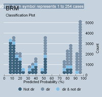
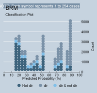
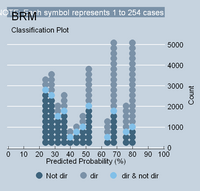
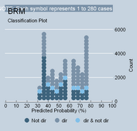
One final observation. Below are the classplots from four regressions I have recently discussed: (1) the autonomy model; (2) the small dependency model; (3) the large dependency model; and (4) the model that exists in reality. Recall that in reality newspaper reputation is not an especially good regression by any means. It has a likelihood-ratio R-squared of only 0.067 and explains about 24% of the overall voting variance. It’s KDV is also only 41%. The reason why each of these models is different can be clearly seen in the classplots below. In the autonomy model, the polarizing voting is creating an ideology model that belongs in "attitudinal" heaven. As the extreme-valued justices are squished inward, the models begin to lose their anchors. Also, as more and more justices exhibit non-directional voting patterns – as they begin to congregate around the 50% range – the model simply becomes “clogged.” Take a look yourself:

<--Autonomy Model   <--                                                                                                                Small  Dependency

<--Strong Dependency  <--                                                                                                                  Reality

[1] It is important to remember that the KDV reports a sum of all of the changes in the predicted Y as X increases from its minimum to maximum in 10% increments. The discreet change in Y for each 10% change in X is symmetrical but not equal. Some 10% changes in X produce larger values than others. Once again, the KDV simply is a sum of the changes.