Ideology Models Only Account for 12.5% of the Votes!

I need to make a clarification about something. On several occasions – both in here, on Howard’s list and on ELS – I stated that newspaper reputation accounts for only 24% of the votes that justices cast in civil liberties cases over the last (almost) 60 years. That figure may be somewhat misleading. I grabbed it from phi-p, which is a correlation statistic used in contingency-table analysis. But whether or not it is misleading, one of the things that is undeniable is that in the ecological regression of civil liberties votes endorsed by numerous political science scholars, only 12.5% of the total votes cast in civil liberties are responsible for the 41% of the variance in the liberal index that newspaper reputation “explains.” Only 12.5%!! Let’s take a closer look.

As I have demonstrated previously, the R-squared in an ecological regression involving Segal/Cover scores and career liberal ratings in civil liberties cases from 1946-2004 is 0.41. Keep in mind that this figure is not the explained variance of the votes; it is the explained variance in the numbers comprising the liberal index. To equate the one with the other is an ecological fallacy. To see just how damaging this fallacy is, I have provided a table which looks closely at what this R-squared statistic is reporting. The table can be accessed here.

The table is useful for several reasons. First, it breaks down the explained and unexplained variance that occurs in the numbers comprising the liberal ratings. It also, however, breaks down the number of justice votes implicated by those percentage points. As one can plainly see, the number of votes that accompany the explained portion of the regression is only 12.5% of the total number of votes that comprise the entire regression (31,049). That means the regression is only able to rely upon 12.5% of the votes to explain 41% of the variance in the ratings.

Another thing that is interesting is how each justice is affecting (or driving) the R-squared. This can be located in the column to the far right, called ERL (Explained Ratings Load). This column is simply referring to the contribution that each justice is making to the R-squared statistic (the explained variance). The justices who are actually driving the statistic the most are the ones who carry the highest proportion of influence (“load”). Scalia is a good example; he accounts for over 6% of the R-squared by himself. Justice Rehnquist is right behind him.

But now, however, examine the column titled EVL (Explained Voting Load). This column shows the proportion of votes that are hiding behind each of these “rating loads.” This is simply the proportion of the 12.5% of the total votes to which each justice contributes. Here we find something else of interest. First, there are, as one might expect, some justices who “artificially” contribute to the R-squared by having “payoffs” in their percentage points that are not matched by their votes. Good examples of this are justices Goldberg, Fortas, Rutledge, Jackson and Thomas (to some extent). To see this better, examine the following graph (the red lines of those justices – the percents – are disproportionate to the grey lines, the votes). Also, of the 12.5% of the votes that are needed to drive the 41% of the ratings, the bulk of the work comes disproportionately from four key justices: Rehnquist, Blackmun, Brennan and Douglas.

I’ll have more to say about this in a couple of days. I’ve got to run now.

What Causes These Ideology Models to Fail?

[Version 2]*

In my last entry, I showed that newspaper reputation for political direction did not constitute as significant or substantial of an explanation of voting behavior as many political scientists had suggested over the last sixteen (16) years. Although its performance may be perfectly acceptable to some, clearly, others in the discipline seem to wish it would be strong enough to explain the bulk of what the Court does in civil liberties cases (which it does not). In this entry I take up the issue of why ideology models do not perform better.

The answer is straight forward: there are simply too many justices who do not affiliate well with the binary outcome being analyzed by the model. If a logit model was a drain, centrists justices are the clog. And that means that “newspaper ideology models” are really nothing other than a partially-clogged piece of plumbing. To demonstrate this, examine the stepwise analysis (Table 5 in my SSRN paper). It begins with the logit results of Segal and Spaeth’s base ideology model, updated to 2004. It then subtracts the justice with a liberal rating closest to pure non-direction (.5) and re-estimates the regression. The subtraction continues one justice at a time until only those justices with ratings above 66.1 (Ginsburg) and below 33.9 remain. The subtraction increment is 16.1 points above or below 50%. As each median justice is subtracted, the values of the regression increase remarkably. At the very end of the regression, Justice Douglas is added. By this time, the only justices remaining in the analysis are the following ten: Brennan, Burger, Fortas, Goldberg, Marshall, Rehnquist, Scalia, Thomas, Warren and Douglas.

The table is simply amazing. The model has been transformed from “clogged plumbing” to Niagara Falls. It now has a KDV of 78 points and increases the ability classify the direction of votes by 57%. The total voting variance explained by the model is also 57% (phi-p). Or, stated another way, “Rehnquist votes the way he does because he is conservative; Marshall voted the way he did because he is liberal.” To really see the effect of “clan voting,” examine the classification plot below. It shows quite clearly why the model performs so well: there are no justices clustered around the 50% mark, and the model has two solid anchors on each side:

What does this show? It demonstrates is that one cannot create a bivariate ideology model that has the level of explanation that Segal and Spaeth originally believed they had created – a model that explains at least 60% of the Court’s choices – without first removing every justice from the truncated model having a liberal rating within 34% and 66.2% (and adding Douglas).[i] What this also says is that scholars who are championing the idea of an ideologically-driven Court are simply allowing the votes of those justices with the most obstinate judicial personalities to stereotype the majority of the institutional-membership’s voting behavior.

To see this, consider the model in Table 6 of my SSRN paper. It analyzes civil liberties voting from 1946-2004, but excludes 8 of the most directional justices having liberal ratings below 23% and over 77% (Rehnquist, Goldberg, Fortas, Douglas, Marshall, Brennan, Murphy and Warren). One of the reasons why excluding outliers is relevant, of course, is that the current Court no longer contains membership with career propensities beyond the values being excluded. Hence, one could argue that this analysis is a better estimation of the degree to which justice ideology governs votes on the current Court, [ii] at least to the extent researchers claim to have observed such phenomena in the Supreme Court data base.

The result of the subtraction is simply remarkable. The index variance explained by the regression drops to 17%. Total voting variance drops to 9% (phi-p), and PRE is only 11% (tau-p). The coefficient in the logit regression indicates that liberal ratings only increase by 8 discreet points as Segal/Cover scores change by 100% (KDV). The classplot in Table 3, Figure 6, speaks for itself. But what is perhaps more interesting is what happens if the subtraction range is increased by one percentage point in each direction (24% to 76%). It results in the exclusion of only two additional justices (Thomas and Rutledge) and produces a statistically-insignificant ecological model. [iii] It is indeed remarkable that an ecological model is completely unable to explain the liberal ratings of nearly two-thirds (22) of the Court’s membership since 1946, and that, whatever level of explanation it otherwise achieves is simply driven by a small minority of the Court’s most obstinate personalities.

---

[i] Some may be tempted to object that this manuscript sets up a test of the attitudinal model that requires justices to vote perfectly liberal or conservative before “attitudinalism” can prevail. This is not accurate. The manuscript merely requires that the career choices of the largely non-directional justices be similar to the directional before the bivariate model can be regarded as systemically dominant as proponents of ecological regression claimed. Indeed, what this manuscript demonstrates is only that what researchers empirically operationalized as “attitudinalism” simply plays a smaller role than previously thought. Finally, it should be remembered that there are three pathways to higher numbers in these models: (a) extreme justices voting with less dependency (see Figure 2 in Table 3); (b) middle justices voting like affiliated ones; or (c) some combination of the two.

[ii] Although the career propensities of Justices Alito and Roberts are not yet known, it is perhaps worth mentioning that both justices are predicted to be in the “moderately conservative” range. Alito’s newspaper reputation for political values was -0.8. His career liberalism is estimated to be 0.355 using a logit model and 0.343 using an ecological model. Justice Roberts’ newspaper reputation, by contrast, was -0.76, making his estimated liberalism 0.364 (logit) and .351 (ecological). However, it must be remembered that these forecasts are not remarkably accurate. The absolute value of the average mistake is 13 points for ecological regression and 13.1 for logit regression. Therefore, one cannot say that Alito or Roberts will not be especially directional. This caveat must be kept in mind when considering whether a regression that excludes outliers is a more accurate model of today’s Court.

[iii] There are other voting circumstances where Segal/Cover scores produce statistically insignificant results in civil liberties cases. Newspaper reputation is a statistically insignificant predictor (p values greater than .1) for every civil liberties vote cast by justices in the years of 1950, 1954, 1964, and 1992 (95% confidence interval, two tailed test). The p-values are also greater than .01 for the years 1949, 1951, 1952, 1953, 1965, 1968, 1991 and 1993 (Wilson 2006).

* substantial edit

The Truth About "Newspaper Ideology" and Civil Liberties Voting, 1946-2004

[Version 2.0]*

I have just spent a week laying out an indictment against the bivariate ideology models that political scientists constructed over the last sixteen years. The indictment is predicated on a basic point: the aggregation of voting data and resulting misinterpretation of the R-squared statistic caused the creation of disciplinary misinformation – empirical falsehoods, plain and simple, that were passed along to political science graduate students and the rest of the academic community. Now is the time to correct these falsehoods by constructing a bivariate ideology model that avoids ecological inference and correctly estimates the relationship between model variables.

First, however, keep in mind a couple of things. I have yet to say anything about the propriety of the measures in these models. Some have said that the stuffing of justice opinions into one of two binary outcomes – liberal or conservative – or the fitting of justices’ preferences in unidimentional space is too simplistic to merit serious consideration. I will visit these issues at a later date. But for now, all that I want to do is find a more simplistic truth: how well do these measures actually perform when researchers model them properly and understand the results?

Below are the results of a logistic regression of civil liberties voting from 1946 to 2004. The regression contains 31,049 votes cast by 32 justices over 58 years of service on the high Court. The data is publicly available from the Ulmer project. [1] Let’s discuss goodness-of-fit first. The first indication that the fit of the model is poor is the rather low value (0.067) of the likelihood ratio R-squared. [2] The second indication that the fit is not that great comes from the PRE measures. Of the three that are listed, tau-p is the best for judicial modeling. [3] Tau-p indicates that the model only increases the ability classify liberal votes by 24%. Also, Phi-p, which is calculated using the logic of Pearson’s r, suggests that the overal variance between Segal-Cover scores and justice votes is about 24% The table can be accessed here.

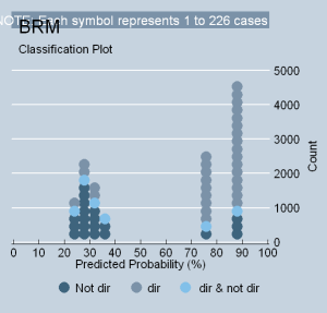
Although analyzing the goodness of fit of a logit regression may not be as easy as an OLS regression, one of the nice things is that both now have the ability to generate a "picture." Take a look at the STATA “classplot” below. It shows why the fit of the model is not very satisfying. The reason is twofold: (1) too many justices are simply “non-directional” (median justices who do not affiliate well with dichotomous choices pull down the model’s fit); and (2) there is not enough “gusto” coming from each end of the value spectrum (no one is predicted to vote in the very extreme ranges of 0 to 29, or 80-100). In short, there is too much traffic around the value of 50% and not enough around 20 or 80. That’s why the numbers are poor.

Now let’s look at the coefficient. I like to focus on what I call the "key" discreet change or value (KDV). This statistic shows the total discreet amount that predicted ratings change as Segal-Cover scores change from their minimum to maximum values. Hence, going from absolute conservatism (-1) to absolute liberalism (+1) -- a 100% change – causes predicted liberal ratings to increase by 41 points, less than half the proportion of the change in values.[i]  Stated another way, newspaper reputation is less than half of the story, even using coefficient logic.  And although these results may be perfectly acceptable to some – they certainly seem to fit a Pritchett framework -- it is quite clear as an empirical matter that they do not: (a) explain the bulk of choices justices cast in civil liberties cases; or (b) establish the mythology of judging by showing the supremacy of political values.   Therefore, the ultimate point is that the reputation a justices obtains for political direction at the time of his or her confirmation does not explain nearly as much of the voting universe as the political scientists who originally constructed or endorsed these models proclaimed. This conclusion is not a matter of opinion; it is true as a simple fact of how data is interpreted and analyzed in a statistical model.

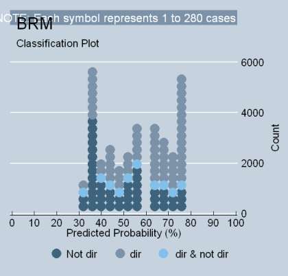
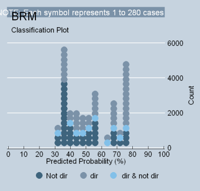
Because some scholars (Segal at al., 1995) believe that ideology models perform better when eliminating justices who predate the Warren Court, it is necessary to consider models that exclude Truman and Roosevelt appointees (the “truncated model”).  The findings are found in Table 4 of my SSRN paper.  It indicates that the truncated model is really no different from the model that contains all of the justices. The fit is poor (0.070 R²_L); the increase in the ability to classify liberal votes is moderate (24%, tau-p); and the total voting variance is about 24% (phi-p). The predicted magnitude of the variable relationship is also roughly equal to a model containing all of the justices (KDV = .418). The classplot below is virtually indistinguishable from the preceding one.  Although it is true that a higher proportion of index variance is present in the shorter list of ratings, only 14.6% of the model votes drive this effect (see Table 8 in my SSRN paper) [ii] and only five justices are responsible for half of it. [iii]  Therefore, the substantive conclusions drawn from a model of a truncated set of justices is really no different from the full model.

REFERENCES:

Menard, Scott. 2002. Applied Logistic Regression Analysis. Thousand Oaks: Sage Publications. 20-27.

Kleckla, W.R. (1980). Discriminant Analysis. Thousand Oaks: Sage Publications. 7-19.

DeMaris, Alfred. 1992. Logit Modeling, Practical Applications. Thousand Oaks: Sage Publications. 53-54.

---

[1] My particular data set is an integration of the Vinson Court data and the original Supreme Court data (updated through 2004). I transformed the data into a single “justice-centered” set with the help of Paul Collins.

[2] R2L is sometimes called “the McFadden R2.” According to Menard (2002), the statistic has the desirable properties of running from 0 (no fit) to 1 (perfect fit), is not affected by the proportion of cases in the sample having the attribute 0 or 1 (called the “base rate), and is not affected by the sample size of the data. However, it is important to remember that R2L is only an analogue to the OLS R2; the two statistics cannot be directly compared. Clearly, R2L underestimates goodness-of-fit when compared to OLS estimations of continuous-level data (DeMaris 1992, 53-54), and cannot be considered itself an explanation of overall voting variance (Menard, 20-24). It is extremely rare, moreover, for a bivariate ideology model to achieve a value of R2L above .4. In the hundreds of bivariate regressions I have performed, I have never seen a value that high. Therefore, I would suggest that researchers involved in bivariate ideology models adopt a simple rule of thumb: R2L values between .2 and .4 are “quite good results” and values below .1 are a baseline for results that are “not so good.”

[3] Based upon Menard’s (2002, 32-34, 36) reasoning, lambda appears inappropriate for a bivariate ideology model because it assumes that errors without the model take the form of an all-or-nothing guess (Menard, 29). In essence, lambda would only be helpful as a PRE measure if modelers could theoretically make the assumption that in the absence of any knowledge of their X variable, every justice in their sample of cases would vote unanimously in every case, the entire sample being all liberal or all conservative. Obviously, this does not appear to be a reasonable assumption.The measure that is best, therefore, for judicial politics scholars is Klecka’s (1980) index originally proposed for use in discriminant analysis models, generally referred to as “tau.” Following Menard’s terminology (2002, 32), I denote the term “tau” with a “p” – tau-p – to indicate its application to a 2 x 2 prediction table generated by a logit model. Tau-p is simply the best PRE statistic for judicial modelers because it assumes that the goal of the logit model is simply to classify as many liberal/conservative votes that are actually found in the base rate of the sample. Therefore, tau-p does not assume an all-or-nothing guessing scenario. It assumes that the number of liberal and conservative votes to be “guessed” in the absence of knowledge about the values of X is simply the proportion of liberal and conservative votes actually present in the sample. In this sense, Menard says that tau-p is less concerned with prediction logic and more concerned with classification logic. (29,33). Of course, like all PRE statistics, tau-p becomes problematic if data becomes excessively skewed.

[i] But how accurate are these predictions? Regressing the predicted liberal score of each justice against the actual ratings produces an R-squared of .4081, indicating that the logit predictions account for roughly 41% of the index variance. (Table 4 lists this statistic as “ppeR²,” which refers to “predicted probability R²”). Note that this is the same amount of index variance reduced in the ecological model. But note also how misleading this can be: As Table 8 shows, the ecological model only uses 12.5% of the Court’s votes to explain 41% of the index variance. And as both the logit model and Table 7 shows, there does not appear to be much overall political direction in the index in the first place.

[ii] Table 8 analyzes the explained and unexplained variance in the ecological model’s R-squared. As one can plainly see, the number of votes that accompany the explained portion of the regression is only 12.5% for the full model and 14.6% for the truncated model.

[iii] Note on Table 8 that only five extreme justices – Brennan, Fortas, Marshall, Scalia and Rehnquist – contribute 56% of the truncated model’s R². When compared to the full model, however, those same justices cannot carry such “loads” – they account for only 37% of the explained variance.

* substantial editing.

Ecological and Logit Predictions of Liberal Ratings

[version 2.0]*

After having my head under the hood of Segal-and-Spaeth’s bivariate ideology model over the last week, I discovered something interesting: ecological regression does not effect how efficiently Segal/Cover scores predict aggregate liberalism on the Court. I had suspected the opposite. Although the two sets of predictors are quite similar and their overall difference is small, there does appear to be one interesting pattern: logit regression predicts liberal justices slightly better while ecological regression predicts conservative justices slightly better. Overall, ecological regression predicted 18 justices better; logit regression predicted 14 better. The best way to demonstrate these findings is by examining the following table and a graph. (Click bold words to access. Look at the output yourself. The graph really shows the story the best. A picture is worth a thousand words).

To explain the findings better, consider the Court’s two newest voters. Just how conservative will Alito and Roberts be? I’ve uploaded another table that analyzes the data.[1]  Alito’s newspaper reputation for political values was -0.8 (see Jeff Segal’s website). That means Alito’s career liberalism is estimated to be 0.355 using a logit model and 0.343 using an ecological model. Justice Roberts’ newspaper reputation, by contrast, was -0.76, making his estimated liberalism 0.364 (logit) and .351 (ecological). In short, both of the new justices are predicted to have a liberal tendency roughly equal to the aggregate tendencies of O’Connor, Kennedy and Powel (to say nothing of the policy differences that will comprise this tendency).

Now the big question: how accurate are these forecasts? The answer is: not incredibly. The average mistake that these forecasts generate is 13 points for ecological regression and 13.1 for logit regression. That means that, on average, Alito could be the next Rehnquist or the next (almost) Stewart. But at least we have a reasonable basis (before he takes the bench) for knowing that he is not the next Stevens or Brennan. Interestingly, if you regress the predictions generated by newspaper reputation against the reality that eventually emerges (the true aggregate liberalism), the R-squared is .4117 for ecological predictions and .4081 for logistic ones. Hence, ecological regression does not affect how well Segal/Cover scores can forecast predictions of an aggregated tendency. But in either case the quality of the forecast that emerges is “partly cloudy.”

---

[1] The table shows not only the difference between ecological and logit estimations, but also the difference between estimations based upon modeling decisions that exclude Truman and Roosevelt appointees versus those that do not. There is some controversy about whether these justices should be excluded. My view is that they should not be. I hope to author an entry about that point later.

* excised unnecessary final paragraph and changed the title.

How Ecological Inference Corrupts an Ideology Model

[version 1.1]*

In my last entry, I demonstrated that the bivariate ideology models constructed by judicial politics scholars over the last sixteen years had the unfortunate property of introducing ecological inference into the regression analysis. One may wonder why scholars did this to their models given the fact that there was no reason to do so (at least not since the mid 1990s). That is a topic for another day, however. For now, I want to consider a more direct question: what is “wrong” with relying upon ecological inference in a bivariate ideology model?

Although there are many problems with models that aggregate voting data, I want to focus upon one exclusive phenomenon in this entry: goodness of fit and model misspecification. I’ll hit the other problems in my next entry.

A. Goodness-of-Fit and Modeling Flaws

The best way to demonstrate the fit problem is with an example, followed by an interpretation. Let us assume that there are two hypothetical courts, Alpha and Beta, each with five justices who have the following voting data: 

Alpha Court:				Beta Court
Justice	N	Pct. L	Segal/ Cover	Justice	N	Pct. L	Segal/ Cover
Rove	10	.10	.10	Rove	10	.10	.10
O’Connor	10	.30	.30	Drudge	10	.10	.30
Stewart	10	.50	.50	“Teddy”	10	.90	.50
Clinton	10	.70	.70	Jesse	10	.90	.70
Nader	10	.90	.90	Nader	10	.90	.90

The difference between these two courts is that one has a distribution of liberal votes that is symmetrical, the other is polarized. The Alpha Court is anchored by two extreme justices, followed by those of proximate distance and a centrist. The Beta Court, by contrast, is plagued with two extreme “clans.” In both cases, however, the hypothetical Segal-Cover scores are the same. That is, in the case of Alpha, the scores correlate perfectly with the percentage of liberal votes cast -- think of it as the attitudinal model in heaven -- but in the case of Beta, newspaper editorials were simply not as accurate of a forecast.

If one were to regress the Segal-Cover scores against the votes in each of these courts, what do you think the difference would be in the goodness-of-fit for an aggregated versus non-aggregated model? The answer may surprise you. In the logit model, goodness of fit is around .5 for the Alpha Court (symmetrical) and .8 for Beta (polarized).[1]  However, in the aggregated model, goodness of fit is a perfect 1.0 for the Alpha court and .47 for Beta.[2]  In other words, the fit of the models is moving in an opposite direction.

And now the critical question: how come the aggregated model cannot properly distinguish between symmetrical and polarized voting for purposes of fit like the non-aggregated model can? That is, how can a model of bias report that a voting universe is less explained by the presence of bias when it is dominated by two extreme clans – the “Rehnquist Five” logic – versus when it has symmetrical variety? The answer is straight forward: when data exists in a binary format, cases that do not affiliate well with dichotomous outcomes – those that show little to no favoritism for “0s” or “1s” – are interpreted as not fitting the model framework well. Hence, Justice Stewart on the Alpha Court is pulling down the model’s fit. However, in an OLS regression of continuous-level data, median cases of X only fail to fit their model if they have extreme Y values (are outliers). Hence, “Teddy” on the Beta Court is pulling down the fit of the OLS regression. (Picture a scatter plot: Teddy is the highest from the line. I have the data posted below if you want to play with it).

So what do we make of this? The point is that the only way a median justice will fail to fit very well into an ecological regression that is already anchored by two extremes is if he or she is so extremely directional (biased) as to be an outlier (Teddy). Yet, if that same voting pattern happens in the logit regression, goodness of fit would increase, not decrease, because the more movement one sees “out of the middle,” the better those models perform. Hence, what aggregation does is it transforms poorly fitting cases in one model into perfectly fitting cases in the other. Stated another way, it transforms non-directional justices into optimally-biased justices.

Given what I have just demonstrated, it should be quite clear why aggregating votes is fundamentally objectionable from the standpoint of both measurement logic and model specification. Quite simply, a model that transforms median justices who do not affiliate with an observed measure of bias into cases that actually “jack up” the model’s assessment of how well bias explains the voting universe is nothing other than a kind of sophistry masquerading behind statistical software. It is sophistry because: (a) bias is supposed to be an observed, empirical phenomenon, not a manufactured one; and (b) a model predicated upon the idea that a median-measured justice could lower the overall picture of bias in a voting universe by becoming an extremist is simply an invalid theoretical design.

Some might be tempted to argue, however, that non-directional justices have “moderate ideology,” and that this is their true “bias.” The argument would be that aggregation is good because median-measured justices should bolster fit unless they become extreme. The reply to this view is straight forward: Segal and Spaeth do not have a criteria for observing moderation as a political subject matter at the case level. That is exactly what the whole objection is. What is a vote for moderate ideology? To determine whether non-directional justices are, in fact, expressing preference for a political subject matter that is different from liberalism or conservatism, one would need to observe it with a trichotomous variable that provides acceptable coding criteria for the three distinct ideological choices. Or, one would need to create a continuous level measure of quality liberalism for each choice available to a justice (McGuire and Vanberg). To date, neither of these options have materialized. Even if they ever do, it is doubtful that such an innovation will help the fit of ideology models. The reason is that the justices who we think are liberal and conservative may “defect” quite regularly for centrist alternatives. If this happens with any regularity, the goodness of fit will not be as high as some in our field would like.

Therefore, transforming justices who systematically resist a measure of bias into perfectly-biased justices through the magic of aggregation is a most objectionable way to conduct empirical analysis of the data that is currently available. In short, these ecological models are misspecified.  No longer can political scientists assert as an empirical matter that 60-to-80% of the choices justices make in civil liberties cases arise out of their political values -- at least not to the extent that researchers have observed such phenomena in a data set. There is absolutely no empirical truth in that assertion whatsoever.

OUTPUT FOR ALPHA AND BETA: 

The STATA file:  http://ludwig.squarespace.com/storage/experiment.dta;  Goodness-of-fit tables for the logistic regressions: http://ludwig.squarespace.com/storage/table.alpha-beta.doc

REFERENCES:

McGuire, Kevin T., and George Vanberg. 2005. Mapping the Policies of the U.S. Supreme Court: Data, Opinions, and Constitutional Law, paper presented at the Annual Meeting of the American Political Science Association.  

---

[1] Logit is estimated with maximum likelihood. The only way to achieve a 1.0 (perfect) goodness of fit in a logit model is if the classification table perfectly predicts complete polarization. There would be no classification errors whatsoever.

[2] For those wanting more information, the logit classification table appears at the end of this journal entry. Fit is assessed with the R-squared analogues of phi-p and tau-p.

* corrected the spelling error in the title; minor editing in the final paragraph.