This area does not yet contain any content.
Thursday
Sep212006

Colonial Williamsburg is Biased

I am shocked at how biased Colonial Williamsburg is. It is no more a display of American history than it is a display of parochial anti-federalist political culture -- which is, at best, only a factious component of both American history and the revolution.  I was stunned to find out that Washington's stature was demeaned while Jefferson's was artificially enhanced. I was stunned to have one of the tour guides in uniform tell me that Peyton Randolph would have beaten Washington to become the first president of the United States in spite of Washington stature after the war, had Randolph merely lived. I was also stunned to hear one of the tour guides tell me that Virginia is really the most relevant place to spend the 4th of July in America and not Philadelphia. The rationalization for this nonsense was the fiction that Virginia was ahead of Philadelphia in the push for independence. We all know, of course, that if any American or locality was pushing independence before the others, it was Adams in 1775 (in Philadelphia) and elements in Boston who were the first to face gunpoint.

But aside from telling me lies about American history, perhaps the most egregious myth in Colonial Williamsburg is what is not told. Nowhere is Alexander Hamilton mentioned. Hamilton, of course, was the general in Washington's army who led the battle of Yorktown, which, the last time I looked, was in Virginia. And that means that somewhere near the time of the battle of Yorktown, Hamilton would have slept in the Wythe house in Colonial Williamsburg, along with Washington and the rest of his generals who used the house for a brief stay. Why is it that no monument to Hamilton is present on these grounds? Why do they mention Washington's presence in the home but not Hamilton's? Why is John Marshall not mentioned? He was a Virginian who was at Valley Forge and later created the most important Supreme Court ruling in United States history. Surely, he walked the Williamsburg grounds somewhere.

I'll tell you why they are not mentioned: they are federalist. The same mischief that promotes Jefferson and makes Washington an after-thought also excludes Hamilton and John Marshall. You are lucky to get anything but a pair of funny glasses in the name of Ben Franklin.  It is one thing for Virginia to be so arrogant as to display only its native sons as an advertisement for all that was most important in the birth of America;  it is another thing, however, to construct those sons so that federalists are either demeaned (Washington) or excluded (Marshall).  It is still another thing to take a key American figure who commanded the winning revolutionary battle on Virginia's soil, spent the night in Williamsburg and eventually constructed finance capitalism in America -- and to say absolutely nothing about him in the town where his American adventure passed. If Colonial Williamsburg wants an anti-federalist propaganda show for its vacation spot, so be it. But if it wants more than a parochial view of history -- if it wants what it advertises to non-Virginians who decide to visit -- it should stop peddling historical lies and a one sided view of what the American revolution was all about.    

Saturday
Aug192006

What About the "Case Facts" Model?

[shared knowledge]

I want to briefly discuss another kind of "attitude model" that is often appealed to by political science scholars.   It combines what its creators call “case facts” with measures of ideology into a multi-variate analysis of discreet areas of voting (e.g., search-and-seizure) (Segal and Spaeth 2002, 312-320, 324-326; Segal 1984). This model is called the “case-fact” model.

As others, however, have noted (Friedman 2006, 268), it is regrettable that the variables in these models are actually called “case facts.” In the case of Segal and Spaeth's (2002) search and seizure analysis, for example, the variables are probably better understood as circumstances that have been recognized by the Court to morally guide the process of intrusion. For example,  what is said to be a "case fact” is whether the search is “incident to arrest;” involving warrants, probable cause and warrant “exceptions;” and occurring in the house, car, person or business (314-318).  Obviously, the Court has created legal doctrine that specifically prescribes the propriety of police intrusion under of each of these searching circumstances. It really should not be surprising that a statistical model could be created that extracts searching-guideline criteria from doctrine announced in prior cases and then demonstrates that the criteria is a statistical predictor in the very cases where the doctrines were created or enforced. Simply labeling the  announced circumstantial criteria governing the propriety of a search as “facts,” and then claiming that justices vote in cases based upon "the facts," does not allow one to escape the circularity problem that such variables really measure a doctrinal construct and  “conclusions of law.” (Friedman, 268).

A more general problem is that “facts” themselves are rarely judged by appellate tribunals. It is the trial courts that judge the facts (innocent, guilty). That is the reason why trials frequently culminate in a document titled Findings of Fact. The appellate courts, on the other hand, harvest the already-judged facts into a prudential construct. To see this, consider once again the search and seizure example (318). Although Segal and Spaeth argue that what influences voting is the “fact” of where the search occurred (person, place, business, home, etc.), the reality is that the Court is organizing instances of the behavior of intrusion via comparison and contrast to form a Constitutional “meta-doctrine.” What emerges, then, is a prescriptive order about the propriety of intrusion that could probably be called the “territoriality theory" of Fourth Amendment jurisprudence. This theory says, quite simply, that your privacy rights are substantial in your home but not out in "public" (which is why the location of the search is a statistical predictor). Hence, what is being voted for is the construction of a theory of territoriality that governs a set of searching circumstances and that serves as a sort of a “meta-doctrine” for the whole area of Fourth Amendment jurisprudence. Segal and Spaeth, therefore, really do not have a true “case facts” model; they have a model that catches the residue or "particulars" of a doctrinal construct and then purports to predict the outcomes of searches in the very cases where the construct was created or enforced. The problem is as much about tautology as it is vocabulary.

So does that mean that judges never "judge facts?"  Of course not.  For a jurist to be truly a judger of facts, he or she must make a decision based upon an attribute of a case that is unrelated to legal doctrine.  For example, let us say that a trial judge has to decide how many bloody crime-scene pictures to allow into evidence under the prejudice-versus-probity rule. Because this rule is governed by the abuse-of-discretion standard, there is really not much "law" (as in rules or -- I would argue - meaningful standards) to dictate the decision. The judge is generally free to let in any amount -- or even differing amounts --  of photos he or she desires. Let's say that Judge Judy has two murder cases, A and B. If she admits extra gruesome crime photos for Case A because it is a high profile case involving someone from a wealthy neighborhood, but admits a lower number for Case B because it is a poor neighborhood, that would be an example of using attitudes to judge facts. It would be judging facts because there is no evidence of doctrine sanctioning the "neighborhood-value" theory for the admissibility of crime photos. The judgment is therefore made based upon facts that were never woven into a prudential construct. Neither Judge Judy nor her peers are obliged to follow this criterion when judging photos in the future.

How would an appellate court "judge facts?"  One way would be agenda access. If a state supreme court justice votes to place cases on the docket more often for campaign contributers than otherwise, that would be a ruling based upon facts unrelated to doctrine. The Supreme Court might engage in such behavior if it decided a case based upon a "concealed fact" -- i.e., a fact that was not processed into the explicit doctrine. Let's say that the Court strikes down a sodomy law using rational basis instead of strict scrutiny because, if it uses higher level review, it may have to strike down certain marriage laws as well. (Lawrence v. Texas).  If the rational basis law stays weak in all other contexts, the Court will have "judged a fact" unrelated to doctrine.    

So I guess the ultimate point is this:  when supreme court judges make decisions on the merits, they do not generally "judge facts." They process already-judged facts into a construct that explicitly defines the propriety of the activity in question (e.g., searching).  This is not to say that this process is or is not ideologically driven. For search and seizure, it may well be. It is only to say that Segal and Spaeth's "case facts" model suffers from the objection of tautology, vocabulary and theoretical design.  It cannot be relied upon to demonstrate that judging is mythical or driven primarily by political values.  And it doesn't even show the extent that the justices actually judge "facts" apart from "law" (doctrine). 

Saturday
Jul152006

What if Justices Really Voted Their Values?

In my last two entries, I demonstrated that Segal/Cover scores are an especially directional set of preference assignments that declare some justices to have perfectly-extreme political views. For example, Antonin Scalia is said to have a reputation for perfect conservatism (-1). Through a roundabout way that I will not repeat here, however, I argued that when newspaper editorialists all agree that Scalia is conservative, they do so under the assumption that the political values in question will be expressed within the constraints of a pre-existing institutional environment. Hence, when all the editorialists describe Scalia as conservative, the resulting perfection in the Segal/Cover score does not mean that Scalia is the most conservative individual the planet knows; it means that he is unanimously conservative within an “institutional” framework and an expected set of bounds. In that sense, I said that Segal/Cover scores are a dependent rather than autonomous set of preference assignments.

Today I want to continue the thought experiment that I began in the entry titled, “5.0: What if Segal/Cover Scores Were Perfect?” In that entry, I showed that if Segal/Cover scores were an autonomous set of preference assignments containing no measurement error, justices having extreme beliefs would have created a highly polarized, clan-driven Court in a world where only political values mattered and the constraints of a judging environment did not exist. I want to refer to that regression as the “autonomy model.” However, I did not consider what my hypothetical world would look like if Segal/Cover scores were, in truth, only a dependent set of preference assignments. How would an institutionally-contextual extremist vote if his or her values were already influenced by a pre-existing cognitive edifice and bargaining structure? To answer this question, I conduct two regression analyses below which I call “fixed-effects” regressions (or “dependency models.”).

Recall that my autonomy model required a one-to-one correspondence between scaled Segal/Cover scores and liberal percentages. (This was the assumption that was problematic for some and necessitated the present detour). The two dependency models I construct below shed this assumption in favor two others. The first dependency model assumes that that extremist justices can only have a range of liberal scores symmetrically matching the most extreme-rated justice in the real world (Goldberg). Because Goldberg reached 90%, I assign all justices with a +1 score a liberal rating of 90%, and all those having a -1 score a rating of 10%. The values are scaled accordingly by the simple formula .5 + (score*.4). I call this my “small dependency” model. In the second regression, I confine extreme-rated justices to career-liberal percentages of 20% and 80%. (You will note that this is an especially forgiving assumption inasmuch several justices in the real world have ratings above 80% -- Douglas, Fortas, Marshall and Goldberg). The values are scaled accordingly by the simple formula .5 + (score*.3). I call this regression my “large dependency” model.

The results for both regressions are found in the attached table. I want to discuss the small dependency model first. As one can plainly see, the small model still provides quite pleasing results (although it is not as perfect as the autonomy model). It has a likelihood-ratio R-squared of 0.2281 – a very good number for a bivariate ideology model – and it reduces the error of classifying votes by 48% (tau-p). It explains about 47% of the overall voting variance according to phi-p. The regression coefficient is also strong. The KDV indicates that as Segal/Cover scores go from -1 (perfect conservative) to +1 (perfect liberal), the discreet change in the predicted liberal rating is .955. Once again, that is almost a perfect overall relationship.[1] The only difference between the autonomy model and the small dependency model, then, is that goodness of fit has dropped slightly (from about 59%) and the KDV is barely lower (from about .999).

Now I examine the large dependency model. As the extreme-valued justices begin to be “squished” into the 80-20 parameter, the model begins to lose some of its potency. It has a likelihood-ratio R-squared of 0.1235 and reduces the error of classifying votes by 35% (tau-p). It explains about 35% of the overall voting variance according to the logic of phi-p. Note that the regression coefficient has lost some of its knock-out punch. The KDV indicates that as Segal/Cover scores go from -1 (perfect conservative) to +1 (perfect liberal), the discreet change in the predicted liberal rating is .707. Although this is still a very good number indeed, it is interesting to note that as justices become “squished” even within a model where scores perfectly match percentages, the coefficient loses its near-perfect relational quality.

Also, keep in mind that this model still assumes that Segal/Cover scores have a perfect correlation with liberal percentages under the assumption that the percentage is a function of .5 + (score*.3). If we were to take the values of the independent and dependent variables and plug them into an ecological regression, the R-squared would be a perfect 1.0. In every regression, in fact, where there is a perfect relationship between Segal/Cover scores and percentages, the value of the R-squared is always 1.0. I bring this up only to show you that the R-squared in an ecological regression is a deficient measure. It cannot discriminate between a model showing autonomy in justice values or a model showing either small or large dependency in those values. Note also that in all the hypothetical voting models so far, the coefficient is statistically significant. Hence, if justices really did vote as an autonomy model suggests – or as a small or large dependency model suggests – each time the result would be an ecological model with statistical significance at .000 and a perfect R-squared.

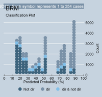
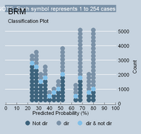
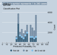
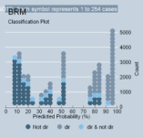
One final observation. Below are the classplots from four regressions I have recently discussed: (1) the autonomy model; (2) the small dependency model; (3) the large dependency model; and (4) the model that exists in reality. Recall that in reality newspaper reputation is not an especially good regression by any means. It has a likelihood-ratio R-squared of only 0.067 and explains about 24% of the overall voting variance. It’s KDV is also only 41%. The reason why each of these models is different can be clearly seen in the classplots below. In the autonomy model, the polarizing voting is creating an ideology model that belongs in "attitudinal" heaven. As the extreme-valued justices are squished inward, the models begin to lose their anchors. Also, as more and more justices exhibit non-directional voting patterns – as they begin to congregate around the 50% range – the model simply becomes “clogged.” Take a look yourself:

586284-394320-thumbnail.jpg<--Autonomy Model  586284-394316-thumbnail.jpg <--                                                                                                                Small  Dependency

586284-394315-thumbnail.jpg<--Strong Dependency  586284-394314-thumbnail.jpg<--                                                                                                                  Reality

[1] It is important to remember that the KDV reports a sum of all of the changes in the predicted Y as X increases from its minimum to maximum in 10% increments. The discreet change in Y for each 10% change in X is symmetrical but not equal. Some 10% changes in X produce larger values than others. Once again, the KDV simply is a sum of the changes.                      

Friday
Jul142006

What Are Segal/Cover Scores Measuring Anyway?

In my last journal entry, I discussed the topic of what reality would look like if Segal/Cover scores perfectly predicted an aggregate voting tendency. Instead of matching the scores to the percentages, I was interested in matching the percentages to the scores. So I constructed a model that was based upon a one-to-one correspondence between scaled Segal/Cover scores and resulting liberal percentages. The model showed, in essence, that the Segal/Cover index is an especially directional set of preference assignments that, if taken “literally,” contemplated a strongly polarized Court driven by “clan voting.” A serious objection to the model was mounted, however. Although it is true that the scores of some justices indicate extreme directional propensity in their political views, it is simply ridiculous to assume that justices having perfect conservative or liberal reputations would never cast a vote contrary to their assigned label in all the civil liberties cases decided during their career. And this is true, the objection said, even in a hypothetical world where only “political attitudes” mattered and no measurement error existed on either side of the regression. Today I want to deal with the implications of this objection.

To have a focused discussion of what this objection really says – and I believe it does say something revealing – it is important to have a clear understanding of what my hypothetical regression assumed. Yesterday’s model assumed a judicial world with the following four attributes: (a) only political attitudes governed judging (the “political assumption”); (b) Segal/Cover scores were perfectly accurate in capturing the directional propensity of those attitudes (“perfect measurement assumption”); (c) the dichotomous coding construct used by political scientists for the model’s dependent variable accurately captured the political choices of the justices (“perfect coding assumption”); and (d) the political attitudes of justices did not change over time (“stability assumption”). If all of this were true in a hypothetical world, why wouldn’t the absolutely biased justices always vote according to their label? (Remember that in the real world Goldberg voted 90% liberal).

Interestingly, I can think of only two answers to this question. The first comes from game theorists. Quite simply, strategy, coalition building and fear of sanction would cause defection from what is maximally desired in the short run in favor of obtaining optimal desires for the long run. In short, justices would occasionally cut their losses in order to obtain a better tomorrow. I will refer to this notion as the “policy game.” The second answer to the question is a little tricky. It says something that seems to violate “the political assumption” listed above, but is actually clever enough to avoid doing so. It says that when newspaper editorialists make claims of extreme political propensity, they simply do so under the assumption that the values being described in the editorials can only be expressed within a preexisting “judging context.” That is, when editorialists say that a nominee is "liberal" they probably assume that he or she will express a relative preference for liberal social policy within the context of the judging environment. Note that this does not say that there is measurement error in the scores; rather, it says that a score of -1 (perfect conservatism) or +1 (perfect liberalism) is simply an indication of a contextual extremity. Hence, that is why one cannot assume a one-to-one correspondence between scaled Segal-Cover scores and aggregate career voting even for an attitudinal model in heaven.

But if either of these options is true, something rather revealing has just occurred. Did you catch it? Because both the “policy game” and the argument-from-context purport to have their effect upon judicial votes during and as a result of the process of judging, Segal/Cover scores can no longer be theorized to be an autonomous measure of political values. Instead, they must be theorized to be dependent or contingent set of values. To see this, consider Antonin Scalia. Segal/Cover scores say, in effect, that there is no person on the planet who is more conservative that he is. (But in fact, given what I have just said, is it true that the scores say this after all?). If we viewed extreme scores as being a measure of autonomous values – scores unto themselves as they would be outside of an interdependent judging context – we would have to regard a one-to-one correspondence between values and percentages as being a plausible way to theorize attitudinal heaven (given assumptions (a) through (d)). But if we regard extremity as a relative and dependent phenomenon -- being capable of expression only within the pre-existing decision structure – then Segal/Cover scores are no longer a measure of something that precedes the judicial environment. Instead, they are simply an indirect and imperfect way of forecasting what the true career propensity for direction will eventually reveal.

Hence, what I am saying is that those who object to a one-to-one proportionality for an attitudinal model in heaven are actually (unknowingly?) conceding that their independent variable is making a value assignment that is expected only to manifest itself within the preexisting structural edifice and bargaining context of the Legal Complex. By conceding that this pre-existing environment exists, one concedes that the measure of “attitudes” is a dependent phenomenon. Stated another way, one cannot say that newspaper reputation is an unmolested look into the political souls of judges, yet object to a model where the evidence of those souls bears a one-to-one correspondence to career percentages in a world where the souls are King and everything is measured properly.

Now, what this really says, properly translated, is that the true indication of the dependent value system used by justices to decide cases within the framework of a legal and strategic environment is not Segal-Cover scores, but rather is the true aggregate tendency itself. That is, assuming that the coding of the dependent variable is not problematic and that propensity for political values is stable across time (assumptions (c) and (d)), it would seem logical to use career propensity for direction as the true proxy for justice values. However, you obviously could not use career numbers to forecast career numbers – tautologies in a non-Wittgensteinian sense are indeed the worst. But you could regress the liberal index against the votes to ascertain how well that index as a proxy for political values explains the choices of the justices. Here’s the headline: the more leptokurtic the distribution of liberal votes is, the less sexy the model will be in terms of goodness of fit; the more polarized the distribution, the hotter it looks. And although this conclusion is a “tautology” in a Wittgensteinian sense – i.e., it is axiomatic – it is nonetheless a meaningful assessment of how "politics" --  as that concept is observed and measured in a bivariate model -- explains judging choices.

Program note: In the near future, I am going to begin creating bivariate ideology models that use career ratings as a value proxy instead of Segal/Cover scores. But I am not going to do this right now because I am not done with my Segal-Spaeth critique. I have a few more things to show about the inadequacy of newspaper reputation before I move on. When I do change the independent variable, I will change the website topic from “Segal and Spaeth Critique” to simply “Bivariate Modeling Issues” and will begin seeing if repairs can be made to the problems that I have demonstrated in these models. One of the issues I hope to properly address is whether the dichotomous coding construct used by political scientists is truly problematic or not. (You will note I have been dancing around that one).   

Wednesday
Jul122006

What if Segal/Cover Scores Were Perfect?

What would judicial reality look like if Segal/Cover scores perfectly predicted the liberal tendencies of the justices? Just so there is no confusion, note that one might approach a question like this from “two ends.” One could simply change the Segal/Cover scores so that they perfectly matched the career-liberal ratings of justices in civil liberties cases – creating, in essence, a logit model that regresses career percentages against justice votes – or one could change liberal ratings to reflect what Segal/Cover scores purport to say about them (in theory). It is the latter transformation that I will undertake in this entry. (The former will be undertaken later).

To do this one must ask a central question: if justices voted exactly according to their newspaper reputation for political direction, what would that look like? One answer might be that a perfect match occurs when the propensity for bias found in the reputation has a one-to-one correspondence with the propensity for bias found in the actual votes. Hence, perfect prediction might simply be the scaled Segal/Cover scores.[1]  A justice having a Segal/Cover score of 0, therefore, would be expected to have a liberal output of 50% if newspaper reputation perfectly measured and predicted an aggregate directional tendency.[2]  (For those who object that perfect prediction would not exist using one-to-one proportionality, hold off for just a second).

So what would reality look like if Segal-Cover scores were perfectly accurate, using one-to-one proportionality? To answer this question, I have conducted a logistic regression of simulated data for all civil liberties votes cast for all justices from 1946-2004. (The data is uploaded on this website and can be accessed below). It was fairly easy to create the simulated votes. I simply changed the vote distribution of each justice in my real data set so that the proportion of liberal votes matched perfectly the scaled Segal/Cover score. For example, Justice White has 2,307 votes in the data set and his Segal/Cover score is 0 (scaled to .5); therefore, his vote distribution was changed to 1154 liberal, 1154 conservative.

The results of the regression are quite interesting and can be found in the following table. As one can plainly see, this regression is immaculate. They should put it in an attitudinal museum. The likelihood-ratio R-squared is .38, which is an excellent number for a bivariate ideology model.[3]  According to PRE (tau-p), knowing the newspaper reputation of a justice increases the ability to classify votes by 59%. Phi-p indicates that the overall voting variance accounted for by the model is about 59% as well, which is the level of explanation that Segal and Spaeth originally thought they had created with ecological regression. The regression coefficient also supports a rosy scenario. The KDV shows that when Segal-Cover Scores change from -1 (most conservative) to +1 (most liberal), the discreet change in the probability of obtaining liberal votes increases by .9999, a near perfect match.[4]  The only way this model can become better as far as goodness of fit is concerned is to eliminate the perfectly non-directional justices having “neutral” political reputation (White, Whittaker and Clark).

To see why this model performs so well, examine the classplot below. As one can plainly see, the model is superb simply because it is anchored with extreme values for the predicted Y, with relatively little obstruction coming from the middle-range values. In short, there are two distinct voting clans that dominate the model. Hence, if Segal-Cover scores were perfectly true (using a one-to-one correspondence), the reality that would exist would probably best be described with the following statement: “Rehnquist votes the way he does because he is extremely conservative; Marshall voted the way he did because he was extremely liberal.” (Segal and Spaeth, 2002, 86; 1993, 65).

classplot.segcov.heaven.png

There is still one disturbing objection, however: isn’t it ridiculous to have a hypothetical model where Justice Scalia never votes liberal? My answer at this point is to hedge a bit: this was only a hypothetical exercise. Because some may believe that a better model of perfect prediction should be something less than a one-to-one correspondence, I will adjust the numbers tonight and post a second analysis. I’ve got an idea of what to do.

Data: http://ludwig.squarespace.com/file-download/segal-cover.perfectpred.dta

[1] Segal-Cover scores “count” from -1 to +1, which is 200 increments. The liberal ratings “count” from 0 to 100, which is 100 increments. To scale the Segal-Cover scores, simply transform them by the formula 1 – (.5 - (score/2)). 

[2] So long, of course, as the propensity for political direction remained constant in the values of a justice throughout his or her term on the bench, and so long as the dichotomous vote-coding construct used by political scientists accurately captured its subject (a controversial proposition that I have not yet addressed).

[3]. It is extremely rare for a bivariate ideological model to achieve a value of R2L above .4. In the hundreds of bivariate regressions I have performed, I have never seen a value that high. Therefore, I would suggest that at the outset researchers involved in bivariate ideology models adopt a simple rule of thumb: R2L values between .2 and .4 are “quite good results” and values below .1 are a baseline for results that are “not so good.”

[4] The relationship between the discreet change in the probability of Y for each 10% increase in X does not appear to be linear, however. For some 10% changes in X, the discreet change in the probability of Y is more extreme than for other 10% increments. The KDV reported in the table is the sum of all of these changes.